Have you ever tried to shade alternating rows in Excel to discover that selecting and shading individual rows would take a lifetime?
If you have found yourself in this predicament there is a very simple solution. In this guide I will show you how to automatically shade alternating rows in Excel 2011.
The simplest way to automatically shade alternating rows in a spreadsheet is to make them a table.
When you use tables in Excel you will be able to take advantage of not only analytical tools, but also formatting tools that make customizing tables a breeze.
Shade Alternating Rows in Excel
When you use the Table Styles below, the table will automatically include sort fields for each of the columns in the table.

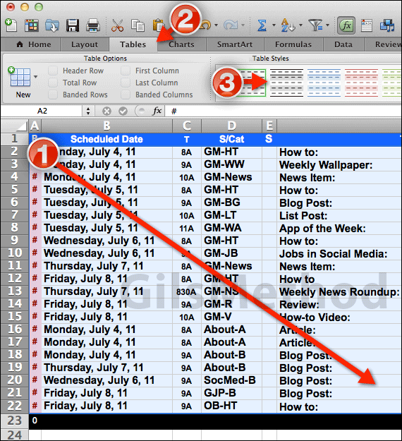
1. Select the range of cells you wish to format using alternating shades for the rows.
Note: Cells can be empty or contain data. Also if you include a heading row, Excel will automatically detect and set it as the heading row.
2. Click the Tables tab on the Office Ribbon.
You will find a slew of tools and options to help you customize your table.
3. For this guide we are interested in Table Styles. Click on one of the available styles to format the range of cells you selected.
You can quickly switch from one style to another to see which you like best.
If you wish to keep the alternating row shading, but not the sort and filter arrows on the column headings follow the additional instructions below.
Remove Table Features

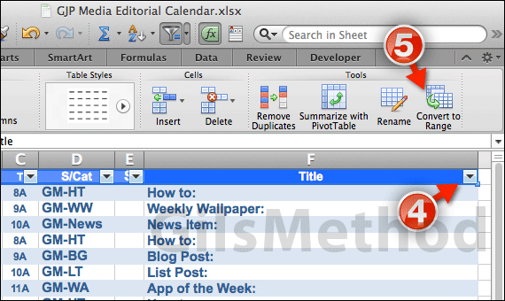
4. Select the table you just created (the range you selected in Step #1).
5. Click Convert to Range in the Tools Group under the Tables tab.
The shading should remain and the other table features should be gone. You have successfully shaded a range of cells with alternating row shades.
Software/Hardware used: Excel 2011 running on Mac OS X Lion.


